[Deep Dive] Does raising a credit limit increase defaults? A test on three public datasets

If you raise someone’s credit card limit, does their probability of default go up or down? Intuition says up. They can borrow more, after all. But open the data and it’s the reverse. This post untangles that paradox with debiasing, tests it on three public datasets, and lands on a conclusion I didn’t expect.

In Part 0 I talked about selection bias. This post is the case where that selection bias meets causal inference head-on, in practice. Causal inference itself gets its own deep treatment later in the Basics series, but here I want to show, a little early, how it actually works on the job. All the code and data are public.

1. Data that runs against intuition

Let’s start with a Taiwanese credit card dataset. It covers 30,000 card customers in Taiwan in 2005, with each person’s limit, their billed amount (balance), and whether they went delinquent the following month (published on UCI). It’s a rare public dataset that carries limit, balance, and default together, which makes it a good starting point. Here I plot the actual default rate by limit bucket.

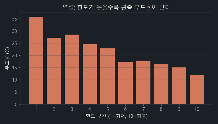
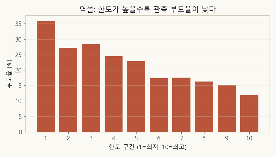
Default rate by credit-limit bucket. The higher the limit, the lower the default rate

The bottom 10% of limits default at 35.9%; the top 10% default at 11.9%. The higher the limit, the steadily lower the default rate (correlation −0.15).

The group that received limits roughly 20 times higher defaults at only about a third of the rate. Does that mean we can hand out limits freely? Of course not. There’s a trap here.

2. The culprit is selection bias

Limits aren’t assigned at random. Under the existing model or rules, high limits go to people who already have good credit in the first place. So “high limit” is really a signal for “someone who was always going to repay.” The negative (−) relationship between limit and default isn’t the effect of the limit; it’s an illusion created by the creditworthiness hiding behind the limit. It’s the most blatant instance of the selection bias we saw in Part 0.

Train a model on the data as-is and it learns “high limit = safe.” Simulate “what if we raise the limit?” with that model and it will tell you defaults go down. Feeding that result straight into a policy decision is dangerous.

3. The fix: turn the limit into a “residual”

The core idea is simple. Compare people with identical creditworthiness but different limits and you can see the limit’s pure effect. Perfect matching is impossible, so instead we do this.

Predict each person’s “expected limit” from their creditworthiness features (X) — that is, imitate how limits were assigned in the first place.
Subtract the expected limit from the actual limit and you get the limit residual (rL): the variation in the limit that creditworthiness doesn’t explain, produced by policy or by chance.
Turn balance and default into residuals the same way.
Build a chain that runs from the limit residual to the balance residual and on to default (the limit → balance → default path).
Because default is 0 or 1, correct the difference in logit space, then add that correction to the initially predicted default probability to form the final value.

Two cautions. First, to prevent data leakage, the residuals must be built with cross-fitting. If you predict a point using itself, its residual shrinks artificially. Second, the more consistent the limit assignment, the rarer people with large residuals are. We up-weight those rare “natural experiment” samples (people with large residuals).

This is the same structure as Double Machine Learning (DML) in causal inference. DML boils down to this: predict the treatment (here, the limit) and the outcome (default) each from the confounder (creditworthiness) with machine learning and subtract those predictions out, then estimate the effect from the relationship between the leftover residuals. The key is to let machine learning absorb the confounding flexibly while using cross-fitting to keep that model’s bias from leaking into the effect estimate. In the end, it’s the job of stripping the confounder — creditworthiness — out of the treatment, the limit.

Before we start, let me flag one limitation up front. The creditworthiness features we control for are only proxies for the true limit-assignment criteria (income, external credit scores, and so on). So debiasing reduces bias; it doesn’t eliminate it entirely. The weaker the control variables in a dataset, the more the negative (−) that remains after removal may still contain bias we couldn’t strip out.

4. Test 1, Taiwan credit card: the bias disappeared, but so did almost all of the effect

Applying debiasing resolved the paradox. Of the apparent −0.15 correlation between limit and default, about 70% was selection bias, and the direct effect left after removal was a small negative (−0.05). That’s the opposite direction from the hypothesis (“limit ↑ → default ↑”).

So where do we test the hypothesis? On a counterfactual: a plot of predicted default rate as we vary everyone’s limit from 0.5× to 2×.

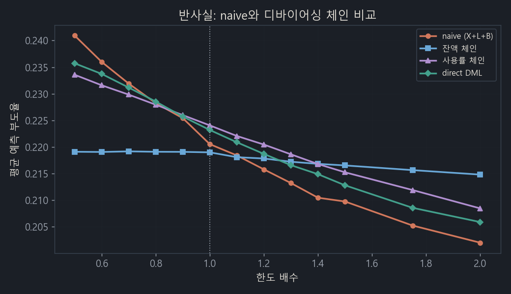
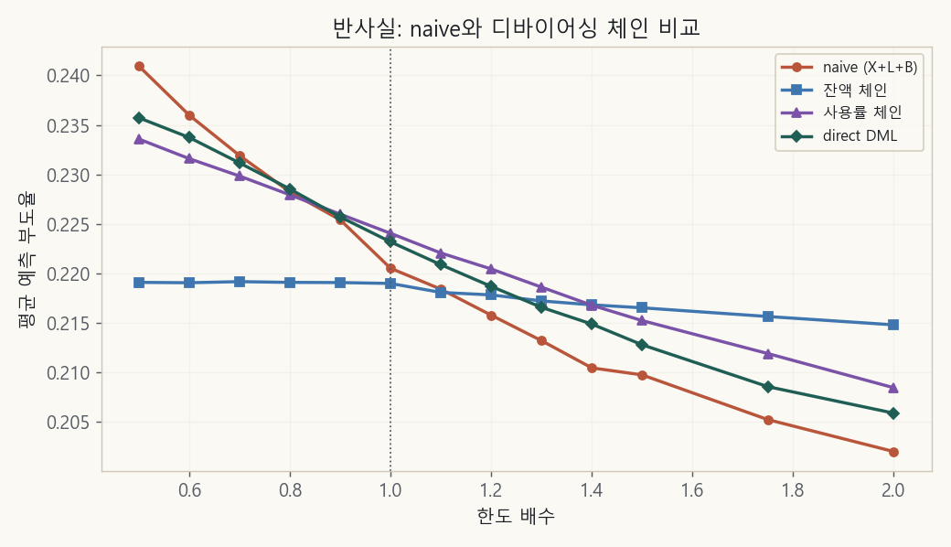
Counterfactual. Predicted default rate when the limit is raised

Red (naive) simply outputs the paradox: limit ↑ → default ↓. The balance chain (blue) goes nearly flat. The utilization and direct chains (purple, green) hold a weak negative.

Analyze it closely and a few things stand out.

Limit → balance is positive (+), but the pass-through rate is a weak 5.7%. That means raising the limit by 1 raises the balance by only 0.057. For an installment loan that’s fully drawn down this value would be close to 100%; against that, a revolving limit is barely used and rarely converts into a burden (it’s sticky).
The real signal of burden wasn’t balance but utilization (balance/limit). And raising the limit actually pushes utilization sharply down (−0.39; it creates headroom).
Isolate balance and estimate it cleanly with a linear model and balance → default is a significant positive (+) (p=0.001), so the hypothesis does hold. The magnitude, though, is tiny.

There’s a methodological lesson here. Use a flexible GBM at a residual stage where the signal is weak and it overfits. Train AUC went up while test AUC actually fell below the base model, and the train-test gap widened to 0.047, six times the base model’s 0.008. The linear second stage that uses residuals only, by contrast, had a gap of just 0.009 — essentially none — and cleanly recovered the true effect. A weak causal signal may be better handled with linear or regularized models.

5. One trap: the observation window is far too short

Default in this dataset is delinquency within “the next 1 month.” Production loss models usually look 12 months out. A short window carries one more bias that heavily affects the analysis: postponement. Someone with headroom in their limit uses that slack to hang on one more month, and their default gets pushed outside the observation window. The default wasn’t reduced, only deferred, yet it gets recorded as “safe.”

This is a separate bias (survival, censoring) that debiasing (removing confounding) can’t catch. I checked it by extending the observation window from 1 month to 5 months.

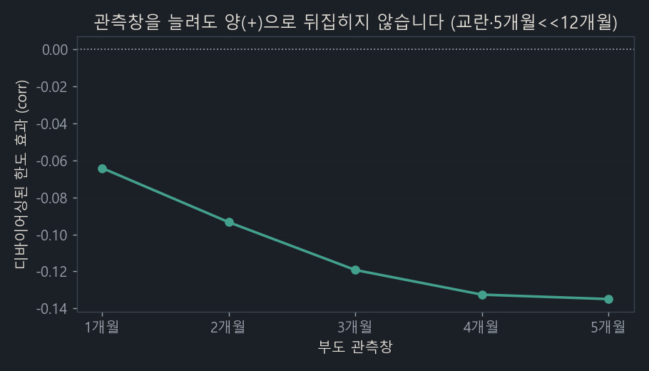
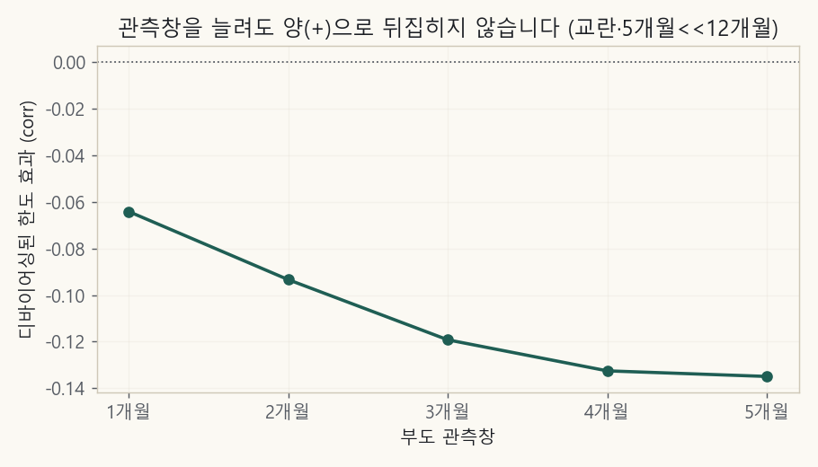
The debiased limit effect as the observation window is extended

Extending the window did not flip the negative (−) to positive (+) (from −0.06 at 1 month to −0.13 at 5 months). That said, in this experiment the longer the window, the thinner the creditworthiness control gets and the more it’s confounded, and 5 months is nowhere near 12. In other words, UCI (1 month) can’t test the 12-month problem.

So I needed genuinely long-horizon data.

6. Test 2, Lending Club: long horizon, and credit that was “drawn down”

Lending Club is a U.S. P2P lending platform. I use 230,000 loans issued between 2007 and 2013 that have already matured. Because they’ve matured, we know the final outcome — paid in full or charged off. Run the same debiasing here and a decisive distinction appears.

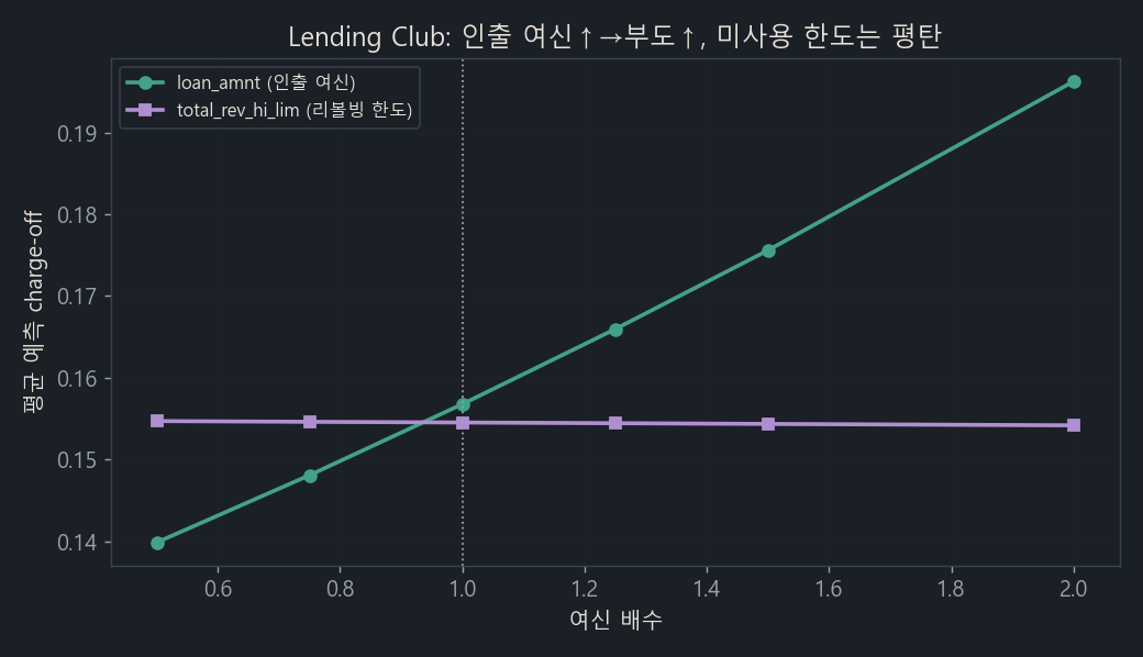
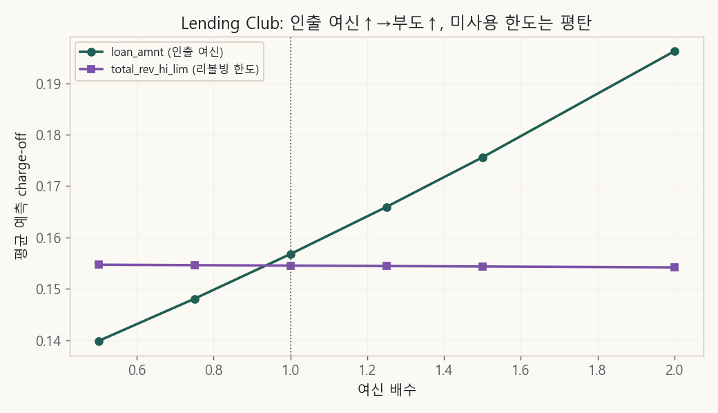
Lending Club. Drawn-down credit and revolving limit

loan_amnt (drawn-down credit, green): even after debiasing, credit ↑ → default ↑ holds cleanly (p<0.0001). It increases consistently across risk grades, and removing the bias actually strengthened the effect. The hypothesis holds.
total_rev_hi_lim (unused revolving limit, purple): even over the long horizon, the effect is close to 0. Just like the UCI limit.

The essence of the difference wasn’t the observation window but “drawn-down credit versus unused limit.” An installment loan is fully drawn down and becomes 100% burden, but a revolving limit isn’t a burden until you draw on it (headroom). The bridge connecting the two is the pass-through rate (limit → balance), and because that was only 5.7% in UCI, the limit effect was weak.

7. Test 3, Home Credit cards: the default definition flips the sign

Home Credit is data released for a Kaggle competition, containing two kinds of records: a monthly credit card panel and application loans (installment). I first tried to nail it down with the card panel — that is, data tracking actual limit, balance, and delinquency over dozens of months on the same revolving product. But the result flipped again. This time it was a warning.

Looking at the roughly 16,000 active cards actually in use, the higher the utilization, the lower the default — the exact opposite direction from UCI. Why?

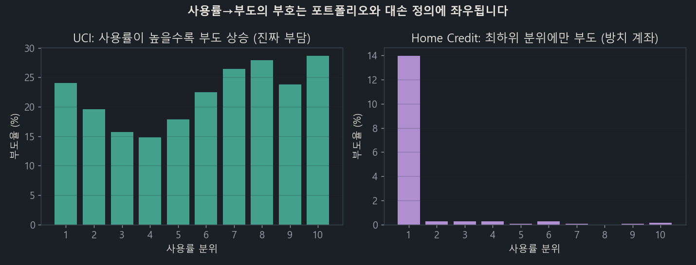
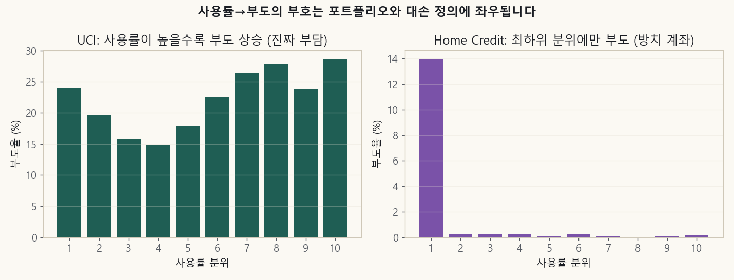
UCI and Home Credit. The sign from utilization to default flips

Left, UCI: the higher the utilization, the higher the default rate (a real burden). Right, Home Credit: default is concentrated at about 14% only in the lowest utilization quantile (balance near 0), while the remaining quantiles sit around 0.1%.

The cause was clear. Home Credit’s “default (SK_DPD≥90)” was capturing not credit burden but dormant accounts that went delinquent because a small balance was left unattended. People who actually use their card default at essentially 0. In other words, when the outcome definition captures “neglect” rather than “credit loss,” no matter how well you debias, the sign flips wholesale.

8. Test 4, Home Credit main loans: the paradox finally flips

Up to this point I’d tried debiasing, but there was no dataset where a paradox that was negative (−) in the raw data flipped to positive (+) after debiasing. And a dataset that met the conditions was sitting right next door: the application loans in the same Home Credit (not the card but the main loan; 8% default rate, 300,000 records). It’s an installment loan that gets fully drawn down, and default here is genuine credit loss. And this time I controlled for the external credit score (EXT_SOURCE) and income together.

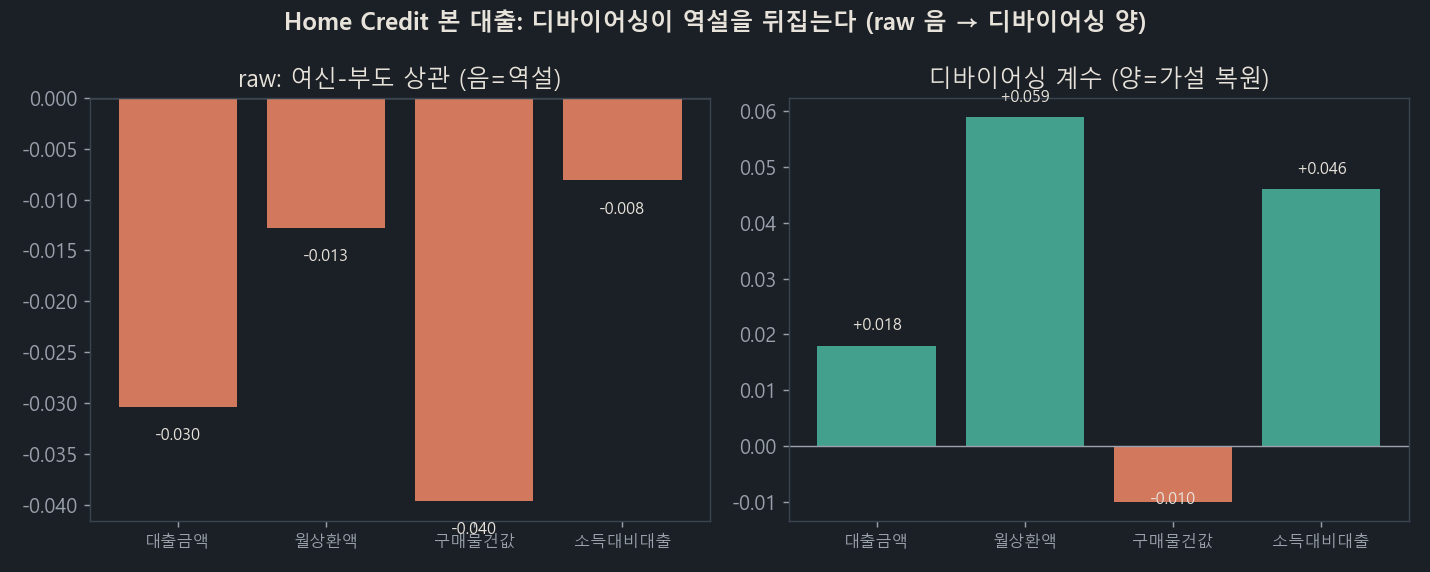
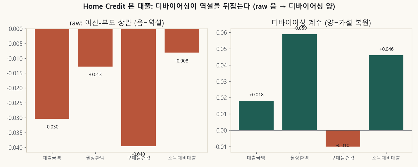
Home Credit main loans. Debiasing flips the paradox

Left (raw): the paradox where larger credit means lower default (all four variables negative). Right (debiased): remove creditworthiness and it flips to positive (+).

Variable	raw correlation	debiased coefficient	verdict
Loan amount	−0.030	+0.018	flipped
Monthly payment	−0.013	+0.059 (p≈10⁻²⁰)	flipped (strongest)
Loan-to-income	−0.008	+0.046	flipped
Goods price	−0.040	−0.010	not flipped

The coefficients in the table are logit coefficients on standardized residuals, so the magnitudes themselves are small. The monthly-payment +0.059 amounts to default odds rising about 6% per one standard deviation. With 300,000 records the p-values are extremely small, but that means “the sign is definitely positive (+),” not “the effect is large.” This post’s claim is about direction (a flip from negative to positive), not magnitude.

Interestingly, only the goods price (AMT_GOODS_PRICE) doesn’t flip. The burden you have to repay is the loan and the payment, not the price of the goods itself, so this matches the theory exactly.

So why does it flip here but not for the UCI or Lending Club revolving limits? Two conditions have to hold at once. First, that it’s drawn-down credit (a real burden that was fully borrowed and spent), so the true effect is positive (+). Second, that selection bias is strong (larger loans go to better customers), so the raw is negative (−). The main loan satisfies both. That’s why the raw is negative, masked by selection bias, and debiasing reveals the true burden effect, which is positive.

9. Putting it together: when does the paradox flip?

Type of credit	raw limit–default	after debiasing	case
Unused revolving limit	negative (paradox)	near 0	UCI, LC, HC cards
Drawn-down credit, weak selection	positive (no paradox)	positive	LC loan amount
Drawn-down credit, strong selection	negative (paradox)	positive (flips)	HC main loan

Cut across the three datasets and two things remain.

“Limit ↑ → default ↑” is not a universal law. An unused limit isn’t a burden if you don’t use it, so its effect is close to 0, and the signs of utilization and balance depend on the portfolio and the default definition.
But the paradox does flip when the conditions are met. Debiasing strips away the false negative (−) and recovers the true positive (+) — but only for credit that can do so (a real, drawn-down burden).

10. So, in practice

Before carrying this result into practice, I want to stress two things first.

One is the limitation. The creditworthiness features debiasing controls for are only proxies for the true limit-assignment criteria, so you can’t declare the residual effect “pure causation.” This is especially true for datasets that lack income or external scores and where reproducing true creditworthiness is hard. Also, this post dealt with probability of default (PD), but production loss rates are often based on loss amounts. Loss amount is mechanically linked to the limit (limit ↑ → exposure ↑ → loss amount ↑), so on the same data the sign can look positive (+). What you set as the outcome changes the conclusion.

So you have to separate the method from the conclusion.

The method (debiasing) is sound and portable. When there’s a genuine positive (+) effect (the drawn-down credit in Lending Club), the method recovered it cleanly. That a negative (−) showed up in other data isn’t a failure of the method but an accurate reflection of the fact that “that kind of credit simply doesn’t raise defaults.”
The directional conclusion is not portable. You can’t use public data to declare “limit ↑ → default ↑ in any portfolio.”
There are two things you must always check on your own data. First, the pass-through rate (dBalance/dLimit): how much a limit increase actually converts into a draw-down burden. Second, the default definition: whether the 12-month default captures genuine credit loss or merely neglect and small delinquencies.

These two decide the sign of the limit effect. Debiasing is only a starting point; the answer is in your own portfolio.

Appendix. Data and reproduction

UCI “Default of Credit Card Clients” (Taiwan, 30,000 records, 1-month delinquency)
Lending Club 2007–2013 matured loans (230,000 records, charge-off)
Home Credit credit_card_balance card panel and application_train main loan (300,000 records, 8% default)
Method: K-fold cross-fit residualization, isotonic calibration, residual weighting, linear second stage (DML). Python (pandas, scikit-learn, lightgbm, statsmodels).
Code and notebooks (Korean and Japanese): github.com/HangilKim11/blog-research

All the figures and numbers in this post are reproducible from public data. The conclusions in the body are about public data; the sign on your own production data has to be checked directly using the two items above.